Time Series - Practical Beginnings

Time Series Analysis

Time series analysis is an often examined topic in actuarial exams and also a cornerstone of actuarial science. Understanding how to work with time-dependent data is essential for any actuary - whether you're analysing claim frequencies, mortality rates or economic indicators.

What is Time Series Analysis?

A time series is simply a sequence of data points collected over time. For actuaries, typical datasets can be as diverse as:

• Monthly insurance claims

• Annual mortality rates

• Quarterly investment returns

• Daily stock prices

The key characteristic that makes time series analysis unique is that the order of observations matters, and there's often correlation between consecutive time points.

Essential Time Series Components

Every time series can be decomposed into several components:

1. Trend: The long-term direction of the data

2. Seasonality: Regular patterns that repeat over fixed periods

3. Cyclical patterns: Longer-term fluctuations without fixed periods

4. Irregular/Random component: Unpredictable fluctuations

Example Time Series in R

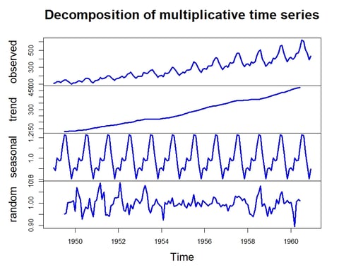
R's built-in AirPassengers dataset contains monthly airline passenger numbers from 1949 to 1960 and is a great example of a time series.

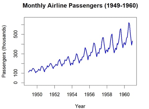
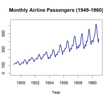
A decomposition of the time series is simple and very informative way to begin, breaking the time series into trend, seasonal and random components. This helps to immediately give insights into what sort of time series it is and how it might be modelled.

Autoregressive (AR) and Moving Average (MA) Models

Understanding AR and MA models is fundamental for time series analysis and is a common actuarial exam topic. These models form the building blocks of more complex ARIMA models.

Autoregressive (AR) Models

An AR(p) model predicts the current value based on p previous values:

AR(1): Xt = φ₁Xt-1 + εt

AR(2): Xt = φ₁Xt-1 + φ₂Xt-2 + εt

Characteristics:

• Values depend on their own past values

• Good for modeling data with memory (like claim frequencies)

• Stationary if |φ₁| < 1 for AR(1)

Moving Average (MA) Models

An MA(q) model predicts the current value based on q previous error terms:

MA(1): Xt = εt + θ₁εt-1

MA(2): Xt = εt + θ₁εt-1 + θ₂εt-2

Characteristics:

• Values depend on past forecast errors

• Good for modeling temporary shocks

• Always stationary

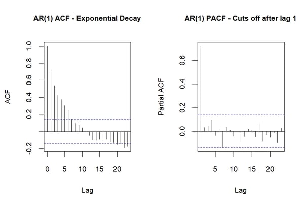
Identifying AR and MA Models with ACF and PACF

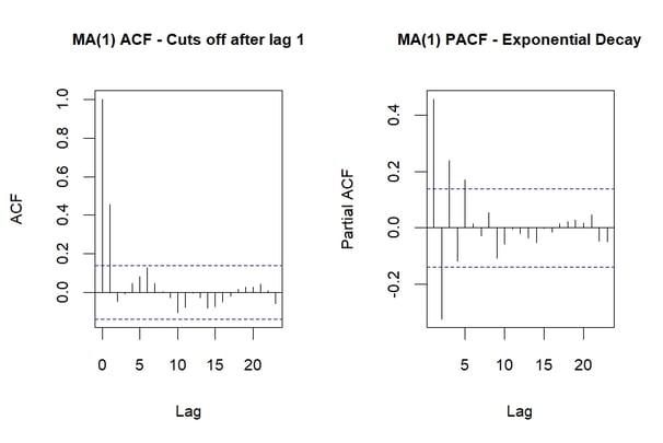
The key to identifying model type lies in the patterns of autocorrelation: